The Case of Rossmann

CS_109 FINAL PROJECT: Rossmann Store Sales Predictions

Predicting sales performance is one of the key challenges every business faces. It is important for firms to predict customer demands to offer the right product at the right time and at the right place. The importance of this issue is underlined by the fact that figuratively a bazilion consulting firms are on the market trying to offer sales forecasting services to businesses of all sizes. Some of these firms rely on advanced data analytics techniques, the kind of which we covered in CS 109. Team "CS_109_Europe" that has been working on this project consists of: Sebastian Fischer, Romain Bui, Zona Kostic. The project is based on data given by this Kaggle competition. You can see our project presentation for more detail:

PROJECT OVERVIEW

Research strategy

To come up with initial questions and to formulate our research strategy, we should first look at the given guidance from Rossmann itself:

Rossmann operates over 3,000 drug stores in 7 European countries. Currently, Rossmann store managers are tasked with predicting their daily sales for up to six weeks in advance. Store sales are influenced by many factors, including promotions, competition, school and state holidays, seasonality, and locality. With thousands of individual managers predicting sales based on their unique circumstances, the accuracy of results can be quite varied. In their first Kaggle competition, Rossmann is challenging you to predict 6 weeks of daily sales for 1,115 stores located across Germany. Reliable sales forecasts enable store managers to create effective staff schedules that increase productivity and motivation. By helping Rossmann create a robust prediction model, you will help store managers stay focused on what’s most important to them: their customers and their teams!

Focus

We will focus our Data Science project on the delivery of a robust statistical model, which is able to accurately predict a 6-week sales performance of Rossmann’s drugstores based on historical data By running through the data science process we will be able to answer the following research questions:

1. To what extend is sales performance influenced by factors like: promotions, competition, school and state holidays, seasonality, and locality.
2. What is an appropriate model to predict sales?

Approach

Our approach follows the generic Data Science process, which was reemphasized in lecture 1 of CS 109. As we just did in the parts above, the process starts with asking an interesting question. With the case of Rossmann we have identified a case, which is interesting for us because the underlying issue of sales prediction is relevant for all kinds of businesses, too. The second step is to get the data. Then, we will explore our data, which is the usual step to take after obtaining data. We will show plots to illustrate properties, trends, anomalies and patterns of the data. After ploting the first results, we will apply different statistical models and compare them to choose the most performing one. Finally, we will answer our initial questions and discuss future research directions.

EXPLORATORY DATA ANALYSIS (EDA)

EDA throught interactive visualizations

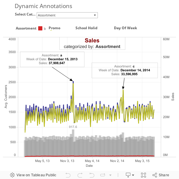
Exploring the given data, we see that Sales performance correlates with the number of customers. The following chart shows the company history of sales (timeline) and customers (bar chart) color coded by different categories. Annotaitons for individual sales based on different categories can be observed with drop-down box.

When looking at the categorical information available for each store, we see that Sales is rather equally distributed over the week. Nevertheless as expected by intuition the amount of customers is higher on weekends as during the week. Furthermore promotional campaigns positively influence sales and the amount of customers.

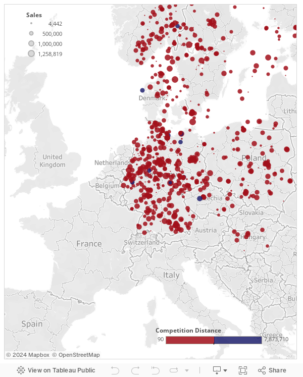
When plotting web-scraped data on a map, one can see that Rossmann’s stores are rather equally distributed over Germany. Furthermore the color code indicated, that there is a rather equally distributed competition distance in place.

FINAL PREDICTIONS

Model

The context consists in the prediction of sales of a shop. We have several variables available including the distance to the competition the availability of a promotion etc. However we can intuitively immediatly think that one of the best predictor for future sales is past sales. We are in a very specific problem where the time dimension is determinant. There is a whole family in statistics: econometric mostly used in finance it consists in properly handling the time series in general. Our approach consisted in a first time in using these tools to perform a first exploration in order to better understand how to handle the time dimension.

The attractive autoregressive(AR) representation

Let's assume that the only data we have are the sales, let's put ourselves in a situation similar to the prediction of a Stock Price where we only know the past observation of the price itself. One could think that if tomorrow is a tuesday, last tuesday is probably a good indicator, how about two tuesday's ago? a month ago? a year ago? We intuitively know that there is an embedded seasonality in the prediction inherent to the calendar. Our though lead us immediately to an intuition on specific time lags that should be more important than other, more specifically a week ago, a month ago, a year ago. This first intuition is important in the process of building the model, since we want to use only the lowest number of dimension as possible to avoid the classical curse of dimensionality.

First steps (EDA again)

To come up with a first modeling approach, we explored the data using an autoregressive correlation approach. From this we saw, that sales can actually be predicted from past sales, because there is a 7-days-seasonability lying within the data.

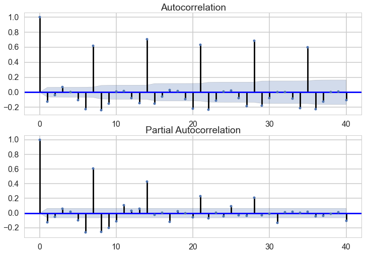
The graph are really obvious, the most important lagged are at 7 days interval, we called these features : d7, d14, d21, d28 for the observation lagged by 7, 14, 21 and 28 days. Looking at the partial autocorrelation graph one can clearly see that the lag predictive power exists until a lag of 28, it disappears afterwards.

The exploration we performed using econometric tools helped us reach important conclusions.

1. The previous observations by themselves are already good at predicting the sales
2. There are key lags to take into account, not all the previous observation have the same explanatory power

Predictions

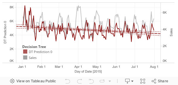
The first model consisted in implementing a decision tree with boosting (AdaBoost). We obtain a very good RMSPE (Root Mean Square Prediction Error) of 0.18, which shows a good improvement in comparaison to the AR model.

A second model consisted in implementing a linear regression, that is obviously simpler than the decision and have a strong assumption of linear dependency. We expected the linear regression to be less good than the decision tree due to this model assumption. However we remind here that our first autocorrelation analysis is based on 'correlation' which is by definition a representation of linear dependency.

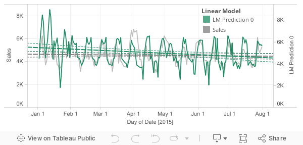
As expected, the linear model gave a poor result of 1.87. and clearly shows in a graphical manner.

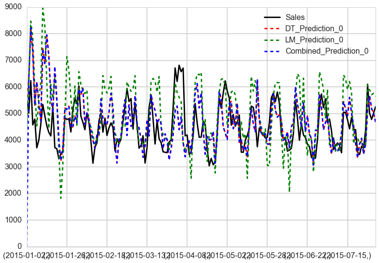
We can see that the baseline model explains the sales pretty decently. Comparing it with the linear and boosted RegressionTree model, we see that the Tree has performed best.

Conclusions

The boosted decision regression tree showed very good results. However we made a convenient circumvolution in the modelisation process. We train the model using d7, d14, d21, d28 therefore assuming that we had this information even in the test sample. The obvious reality, is that we only have the time series feature for the first few observation of the test sample. The prediction process then consists in: do the prediction for the next few days (using the features we have), then use the prediction to update the time series features. Continue this loop until the prediction is finally over. The assumption we make in the fitting process is: 'the prediction we make is the best estimate we have of the future sales'.

Obviously this has a huge snowball effect on the error, the error on the first predictions impacts the next predictions etc. The proper test implementation lead to a poor rmpse of 35, and the graph is as follow :

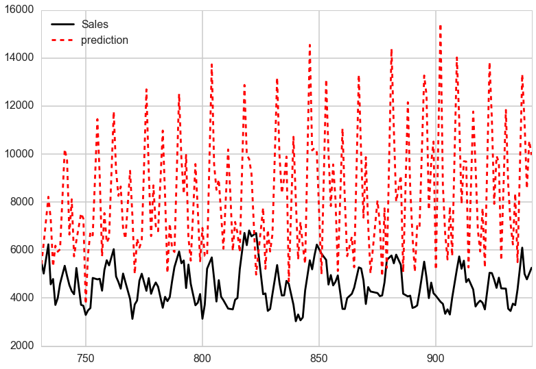
The obvious reality, is that we only have the time series feature for the first few observation of the test sample. We conclude that the time series modeling is challenging because the error builds up when we try to predict the far future. In subsequent research we might want to explore other models that try to adjust for this issue.

The time dimension has a tremendous impact on the approach. When we decided to use the time features (d7, d14 etc.), this means that our predictions are expected to be as good as the in training sample when we predict the next 7 days. Then the build up of the error comes into place.

The Kaggle competition consisted in predicted the next 6 weeks (or 42 days), our splitting lead to have a testing set very large of over 900 days, explaining the fast degradation of the explained variance. These issues are the same the world of finance and economics are facing. For example the usage of an AR(n) to predict future outcomes quickly converge to a stationary states. In a real world, one would adjust the model based on the observed error. This is the spirit of tools such as the 'Kalman Filter' that are usually implemented in these domains.

One other potential approach would consist in implementing more complicated model that naturally combine time series and decision tree, such as ART (Autoregressive Trees).